
When Two TDRs Don’t Agree
As modern high-speed designs push into multi-gigabit and higher data rates, EMI and EMC engineers rely on multiple signal integrity (SI) metrics to evaluate interconnect performance.
Among these, time-domain reflectometry (TDR) remains one of the most direct methods for identifying controlled impedance and discontinuities.
Because impedance mismatch can potentially be a source of EMI, it is important to know the impedance profile throughout the signal path. A TDR plot shows the impedance profile the signal sees as it travels down the interconnect.
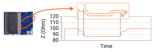
Fig. 1 shows an example of the impedance of a differential pair, and the impedance a signal sees as it travels from the pins of the chip outward.
The impedance of the differential pair is initially higher due to the wider separation of the two traces. The TDR presents a direct method for identifying the impedance and length of the 85 Ohm interconnect.
There are two primary approaches for obtaining a TDR response:
- Measurement in the time domain using a sampling scope, and
- Simulation from measured frequency-domain S-parameters
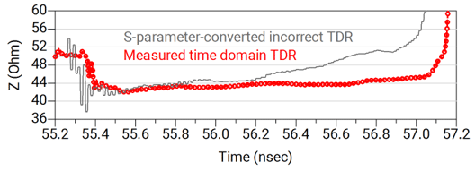
In principle, both methods should yield identical impedance profiles. In practice, differences in S-parameter quality, bandwidth, and simulation setup can lead to noticeable discrepancies (see Fig. 2).
This paper first establishes a structured setup for converting measured frequency-domain data into a time-domain TDR response.
Using an appropriate setup, we then examine various S-parameter properties and their impact on the TDR results. Finally, we conclude with a practical methodology that facilitates a reliable frequency-to-time TDR conversion process.
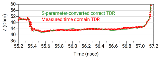
This paper presents a structured workflow for correlating time- and frequency-domain TDR analysis. Using this methodology, a simulated TDR generated from measured S-parameter data correlates with time-domain measurement within ±2.6%, as shown in Fig. 3.
Correlation was evaluated using the maximum impedance deviation between the simulated and the measured trace.
Bridging Two Domains: From Frequency to Time
Whether using a sampling scope or a vector network analyzer (VNA), the objective remains the same: to reveal the impedance profile of the interconnect.
The sampling scope provides a direct time-domain snapshot, while the VNA captures frequency-domain behavior that can be converted to time using a transient simulation.
In a typical TDR measurement with a sampling scope, Fig. 4, a voltage source with a 10-90 rise time launches an incident step into the device under test.
Discontinuities along the interconnect reflect part of this signal, and the reflection monitor at the source records the resulting voltage. From these voltages, the reflection coefficient and corresponding impedance profile are calculated [2].

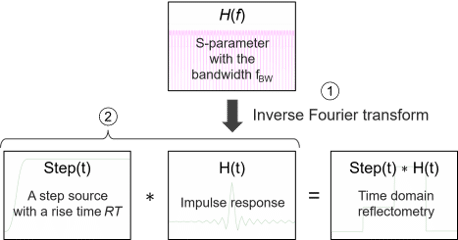
Not every SI lab is equipped with a TDR instrument, but most have a VNA. The VNA’s measured S-parameters can reproduce the same insight by applying an inverse Fourier transform to obtain the impulse response.
During a transient simulation, this impulse response is convolved with the source step waveform to generate the TDR response (see Fig. 5).
Shorter Rise Time Translates to a Higher Bandwidth
In a TDR measurement setup with a step edge, the rise time is an important parameter.
With a shorter rise time, the TDR can resolve smaller physical features that introduce impedance discontinuities. A shorter rise time corresponds directly to a broader frequency spectrum and therefore higher effective bandwidth.
According to the specification of the TDR instrument [3], a source with an 18 psec 10-90 rise time allows the TDR to resolve reflections within approximately a 35 GHz bandwidth, while a faster 8 psec rise time extends the measurable bandwidth to roughly 50 GHz.
The simulated spectrum comparison of the two step edges in Fig. 6 illustrates this relationship: a faster rise time produces a broader excitation spectrum, enabling the TDR to resolve smaller features of the interconnect.
Fig. 6 further illustrates that, in a transient simulation, the step rise time must be constrained by the available S-parameter bandwidth.
If your step source has a rise time corresponding to a 50 GHz bandwidth, S-parameter data with a 40 GHz bandwidth would cause the simulation result to have an unexpected simulation artifact.

The Hidden Influencers: Bandwidth, Step Size, Causality, and Passivity
Because the measured S-parameter data is the focus of the transient simulation, careful examination of the properties of the S-parameter is critical in producing quality TDR plots.
Simulated TDR impedance correctness is fundamentally limited by the integrity of its input S-parameters. The following properties critically influence the outcome:
- Bandwidth: determines the smallest impedance features the TDR can resolve.
- Frequency step: affects the impedance accuracy.
- Causality: ensures correct timing of the TDR.
- Passivity: ensures no energy generation; violations yield higher impedance.
- Reciprocity: less critical for TDR since reflections, not transmissions, dominate the measurement.
Table 1 consolidates the S-parameter properties, their resulting time-domain artifacts, and the practical mitigation strategies required for accurate frequency-to-time conversion.
| S-parameter Property | Time-Domain Symptom | Engineering Interpretation | Corrective Action |
| Frequency step too large | Incorrect impedance result | Poor approximation of frequency response | ≤ 10 MHz step for typical high-speed links |
| Non-causal data | Early arrival, pre-ringing | Violates physical timing constraint | Ensure causality in the calibrated measurement |
| Non-passive data | Artificially higher impedance result | Artificial energy generation | Ensure passivity in the calibrated measurement |
| Non-reciprocal data | Minimal impact on TDR | TDR dominated by reflection | Usually negligible |
Table 1. Mapping between S-parameter property violations and their observable effects in the converted TDR response. Each entry identifies the physical interpretation of the distortion mechanism and the recommended mitigation strategy.
Frequency Bandwidth Determines the Shortest Rise Time
Assume there is measured S-parameter data with a 40 GHz bandwidth. This data is passive, causal, and reciprocal.
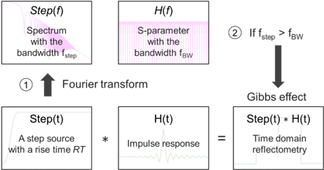
If one simulates this measured data with a 40 GHz bandwidth with a step that has a higher bandwidth (short rise time), one expects the Gibbs phenomenon/Gibbs effect to be present.
Fig. 7 gives a pictorial representation.
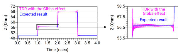
To avoid the Gibbs effect in the TDR result, the step rise time must be short enough to resolve small features, but not so short that it exceeds the S-parameter bandwidth.
Fig. 9 shows the TDR result after simulating a 40 GHz bandwidth S-parameter with a step source that has a correct rise time configuration.

In practice, begin by setting the rise time according to the equation,
RTopt = k/fBW ,
where RTopt is the optimal rise time, fBW is the S-parameter bandwidth and k is the constant that provides the shortest rise time without producing the Gibbs effect.
The constant, k, depends on the transient solver implementation and numerical windowing behavior. Verification that the resulting TDR waveform is free from artificial ringing is important.
In addition to the rise time, when defining the step edge for simulation, it is important to use an edge shape that resembles the actual TDR instrument.
A real instrument’s step edge follows a smooth transition rather than a linear slope. If possible, one should avoid using a linear edge to approximate the transition, as it can introduce unrealistic high-frequency components.
Enjoying this article?
Subscribe to Interference Technology for expert coverage of EMI, EMC, and signal integrity challenges—plus immediate access to new digital magazine issues.
Subscribe here →
Fine Frequency Step Produces the Correct TDR Representation
The S-parameter data represents the frequency response of the device under test. The theoretically correct representation is one with infinite bandwidth and with an infinitesimal frequency step.
In practice, S-parameter measurement produces an approximation of the frequency response because the bandwidth of the data is finite, and so is the frequency step.
Because measured S-parameters are discrete approximations of a continuous frequency response, one expects that as the frequency step becomes sufficiently large, the approximated frequency response of the device under test no longer accurately reflects its behavior.
For the same reason, one expects this wrong approximation to also appear in the TDR response (see Fig. 10).
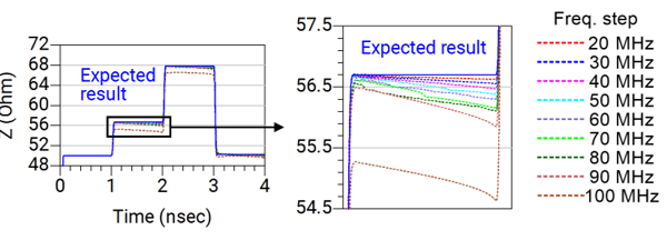
For typical high-speed interconnects, a frequency step of 10 MHz is considered acceptable when capturing S-parameter data.
Non-causality Introduces Incorrect TDR Impedance and Timing
A causal system is a system whose output at any given time depends only on the present and past inputs, not on future inputs. In a causal system, the effect cannot precede the cause.
Interconnects are causal systems, and the S-parameter data representing them should also be expected to be causal.
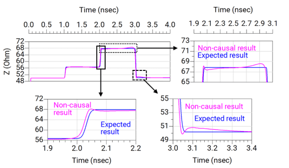
TDR simulation using non-causal S-parameter data will exhibit incorrect timing behavior.
Fig. 11 demonstrates the timing impact of the non-causality in the S-parameter data. The non-causality also leads to erroneous impedance dips and bumps.
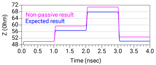
Non-passivity Creates Higher Impedance Readings
When a system is passive, it only consumes energy and does not produce any energy. Interconnects are passive and should not produce energy.
If the S-parameter data violate passivity, the resulting TDR will exhibit artificially higher impedance due to non-physical energy gain.
Fig. 12 confirms the higher impedance when non-passive S-parameter data was used in a TDR simulation. The non-passivity increases the impedance of the TDR.
TDR is not Sensitive to Non-reciprocity
A reciprocal system is one where the forward transmission and the reverse transmission are identical. Interconnects are generally reciprocal.
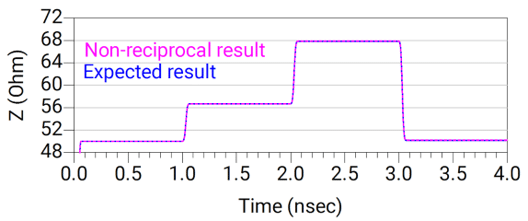
In TDR analysis, reciprocity plays a limited role because the response is dominated by reflections rather than transmission paths.
Because the focus of TDR is on the reflected voltages, rather than the transmitted ones, the TDR result should not be sensitive to whether the forward and reverse transmissions match each other.
Fig. 13 confirms that the TDR simulation with non-reciprocal S-parameter data remains consistent with the expected results.
Shaping Time with Care: Best Practices for Reliable Conversion
Producing a reliable TDR from frequency-domain data requires attention to both the integrity of S-parameter data and the simulation setup. The following practices enable reliable frequency-to-time conversion:
1) Validate S-parameter integrity
Confirm fine frequency steps, adequate bandwidth, and verified passivity and causality. These ensure that the S-parameter model is physically accurate and minimizes simulation artifacts.
2) Use an appropriate step edge
Apply a smooth step that reflects the real TDR instrument’s transition shape. Avoid using a linear ramp, which introduces unrealistic high-frequency components.
3) Match the rise time to the available bandwidth
Select a realistic rise time for the step source based on the S-parameter bandwidth. A practical starting point is RTopt = 3/fBW, followed by waveform inspection to confirm the absence of Gibbs-related ringing.
By following these practices, engineers can confidently generate simulated TDRs that align with measured results, gaining insight into interconnect impedance without needing a dedicated TDR instrument.
Conclusion: Construct the Impedance Profile with Confidence
Time-domain reflectometry remains one of the most direct methods for revealing the impedance profile of an interconnect.
Whether obtained through a sampling scope or reconstructed from measured S-parameter data, the objective is the same: to understand how impedance discontinuities appear along the signal path and how they may contribute to unwanted reflections and potential EMI sources.
While time-domain measurement provides a direct view of this impedance profile, frequency-domain measurements from a vector network analyzer can reproduce the same insight through transient simulation.
The fidelity of the simulated TDR, however, depends strongly on the integrity and properties of the underlying S-parameter data. Bandwidth, frequency step, causality, and passivity all influence how accurately the resulting impedance profile represents the physical interconnect.
By validating these S-parameter properties and configuring the transient simulation appropriately, engineers can generate simulated TDR responses that closely reflect the behavior of the real interconnect.
This enables the discovery of unexpected impedance discontinuities early in the design or validation process, allowing engineers to address potential EMI sources before they propagate through the system.
Acknowledgements
The author would like to thank several industry engineers for insightful discussions that helped shape this work.
References
[1] OpenRex Project, “OpenRex – Open Source Hardware Project,” iMX6 Rex Projects, [Online]. Available: https://www.imx6rex.com/open-rex/
[2] Keysight Technologies, Time Domain Reflectometry Theory, Application Note 5966-4855E, 2004.
[3] Keysight Technologies, “N1055A 2-/4-Port TDR/TDT Remote Sampling Head,” Product Datasheet. [Online]. Available: https://www.keysight.com/us/en/product/N1055A/2-4-port-tdr-tdt-remote-sampling-head.html
[4] R. Baraniuk, et al., “Gibbs Phenomena,” in Signals and Systems, LibreTexts Engineering, 2022. [Online]. Available