An Overview of Coax Limiters for use in HF Systems

OVERVIEW

Critical communication and instrumentation lines subjected to very high energy RF pulses require RF limiters with exceptionally high pulse power capability.

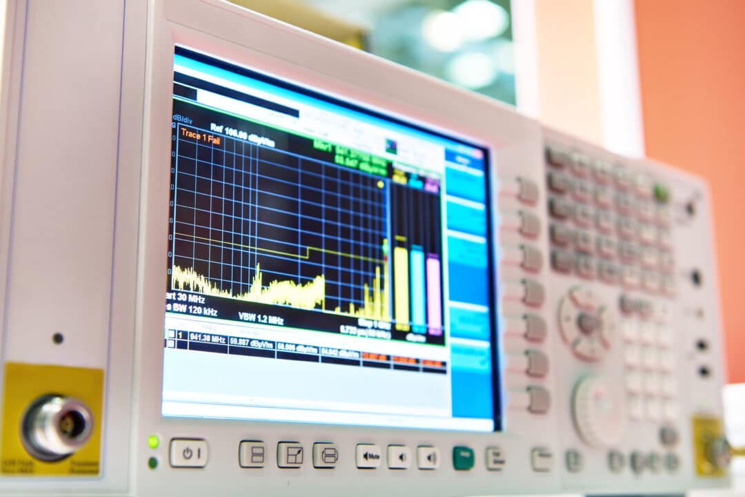
A discussion of a typical high frequency (HF) commercial off the shelf (COTS) limiter manufactured and tested by NexTek is presented to provide insight and understanding of specifications.

Data will be presented from an SMA limiter shown in Figure 1 that has an in-band operating range of 1MHz to 100MHz and is capable of handling pulse RF currents of more than 50 amperes for 10 microsecond pulses.

Bulkhead mountable shielded enclosure approximately 2 inches long with stainless steel SMA Female – SMA Female connectors. VSWR ~1.1; Insertion Loss ~0.5dB with power rating of 20dBm and a max peak pulsed power rating of 10kW at 0.5% duty cycle and 26dBm Flat Leakage.

RF limiters are used to limit the RF power on a circuit. They are also used to protect sensitive receivers from damage due to excessive input power.

Receive circuits, including LNAs, are very susceptible since they are designed for very low-level input signals which are then amplified. In normal operation, the limiter represents low insertion loss to the in-band signal.

However, when there is a higher power level at the input of the LNA (in-band and out-of-band), particularly one that could damage the LNA, the limiter reduces the power level so that the LNA and other components on the receiver are not damaged.

There are several common causes of higher than desired electrical energy on an RF circuit.

These include antenna exposure to high RF fields, which is usually due to colocation or proximity to radar under boresight conditions or other high-power transmitters, RF or circuits that normally handle high RF power, such as manufacturing heating, welding, surface treatment, or non-destructive testing, and environments where there is research using plasma physics, accelerators, fusion, and magnetic diagnostics can present out of band energy that can couple into systems.

The electric field exposure varies by application and environment, and the magnitude of those levels are outside the scope of this discussion.

Typically, an electric field value in V/m is specified by the environment and then a coupling current factor is derived to get a direct current pulsed injection value.

How HIRF exposure direct current injection values are derived are complex in nature and subjective as assumptions and specific systems vary widely.

A simple example of estimating the coupled energy into a system due to lightning strikes has been presented previously (Kauffman & Raina, 1996) and can be used as a guide into more complex electric field coupling calculations.

A commonly high electric field value referenced is MIL-STD-464 Table 2 (MIL-STD-464C) which has an electric field level of 27kV/m fields at 2.7GHz. An exposed antenna could generate over 50kW of power, provided the antenna is rated at or below this frequency.

In other cases, a measurement device might be connected to a circuit capable of similar power.

A limiter should protect the receiver or other instruments exposed to high energy fields that are in-band or out-of-band (10kHz-18GHz).

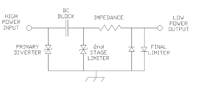
A simplified circuit of a limiter is shown in Figure 2.

The high power enters on the left side and is connected to a primary diverter. This diverter predominately protects the DC block capacitor. This DC block capacitor forms a high pass circuit, defining the lower frequency range of the limiter.

There is a second stage limiter after the DC block. There are further impedances in series, followed by a final limiter stage. This final limiter is shown consisting of two diodes.

The resulting action of the limiter circuit is reducing the RF voltage and power at the low power output side. In general, the stages are coordinated, so that the voltage levels are reduced for each subsequent stage of the circuit.

GENERAL CHARACTERISTICS

Steady State Parameters

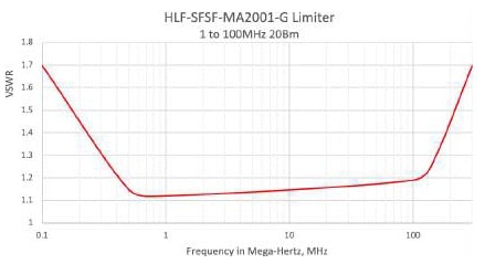
In normal operation, the limiter should have a good VSWR, low Insertion Loss (IL) and not degrade signals that are under the max operational power rating.

However, limiters often have higher insertion loss than typical surge protectors and loses should be included in the systems RF link budget accordingly.

Figure 3 and Figure 4 show the VSWR and IL for the HF and have similar signatures to that of a band pass filter.

DEFINITIONS

Common terms and definitions associated with limiters are presented as an introductory discussion.

Frequency Range: Limiters operation is usually defined by the frequency band.

Some RF parameters, including Insertion Loss and VSWR are not defined out of band, however a good limiter will provide limiting functionality significantly out of band to protect against co-located adjacent band transmitters.

RF Rated Power (RF Watts CW): The maximum power rating in this example is 20dBm.

This level of power is power can continuously flow through the limiter to the LNA. The RF is single frequency and within the operating band.

Insertion Loss: Within the operating band, the insertion loss is usually less than about 0.5dB, this insertion loss is only seen in the operation band and at RF powers below the RF Rated Power rating.

1dB (-1dB) Compression Power: The input power level where the output power has decreased by 1dB from the normal operating loss. This additional signal loss is called signal compression.

Flat Leakage: Indicates the steady state energy that appears at the output of the limiter and is approximately constant.

Spike Leakage: Indicates the short duration and higher level of energy that appears at the output of the limiter that is substantially elevated above the flat leakage region.

Transition Region: The region above the max operat-ing power that includes the 1dB compression point. The transition region starts with the rated power and continues until the limiter is fully activated by high RF energy.

Pulse Operation Region: When the pulse duration for a current pulse exceeds maximum time, requiring pulsing at a maximum duty cycle. This power level is usually about 6dB to 10dB above the rated power.

Flat response is the somewhat steady state output power level, while spike leakage is a much shorter duration output. Since flat leakage is nearly constant, the units used most often are dBm into a 50 Ohm load.

Spike leakage is best referred to as the energy deposited into a 50 Ohm output load and is usually in nano-Joules. Spike leakage can also be reported in peak volts, but this lacks the time element that is captured better in energy.

Pulse Performance

The power transfer function of a typical limiter is shown in Figure 5. There are usually three modes of operation. The continuous operation region up to the rated power level, shown in the figure below as 20dBm (~6.33 Vpeak to peak).

In this region, the VSWR and Insertion loss parameters are substantially constant. As more power is applied, the limiter begins functioning, and the insertion loss can increase by and additional 1dB.

The limiting circuits are just beginning to work at this level of RF voltage. This response is similar to the knee in a Zener diode. The 1dB compression power is usually about 2dB or 3dB above the maximum rated RF power.

The limiter might be operated for the long term at this level of power, but it is not advised, since there is no margin for additional power RF power fluctuations or temperature variations.

When power is dramatically increased, above about 32dBm (~25V pk-pk) the limiter is usually fully functioning.

Substantial increase in input power will have minimal effect on the limited output power. There is a region between the rated power and the full limiting operation, where response is transitional, sharing both characteristics.

High Input RF Energy Response Details

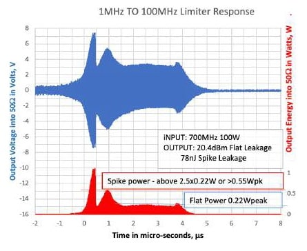
The output response of the 20dBm rated limiter with a 700MHz 100W Signal is shown in Figure 6. The Flat Response voltage is the average of the plateau of power (and voltage) that is about 3.3 Vpeak or about 0.22W peak.

The spike leakage is where the power exceeds the flat leakage by a factor of 2.5, or where the power exceeds 0.55W peak (or the voltage exceeds 10.5Vpk-pk).

The spike leakage signature can vary with different frequency units and can be expressed in terms of power or energy.

The energy curve (in red) shows a well-defined flat leak-age of 0.22Wpeak (20.8 dBm) after about 1.5 microseconds.

A spike leakage is energy above 0.55Wpk, and most energy is confined to the 0.2 to 0.4 microsecond time interval.

A look at the output voltage signatures and voltage levels of the limiter at different power levels provide further examples of transient response characteristics.

Figure 7 through Figure 10 show the output response as the power level increases from normal operation and incremental power increases. A 10usec pulse of 700MHz is used for these increasing power pulses example.

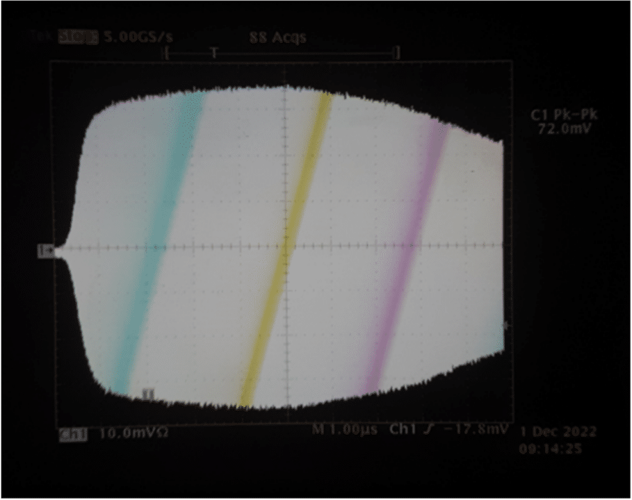
Figure 11 shows the output response of a 10usec 2.2GHz input pulse.

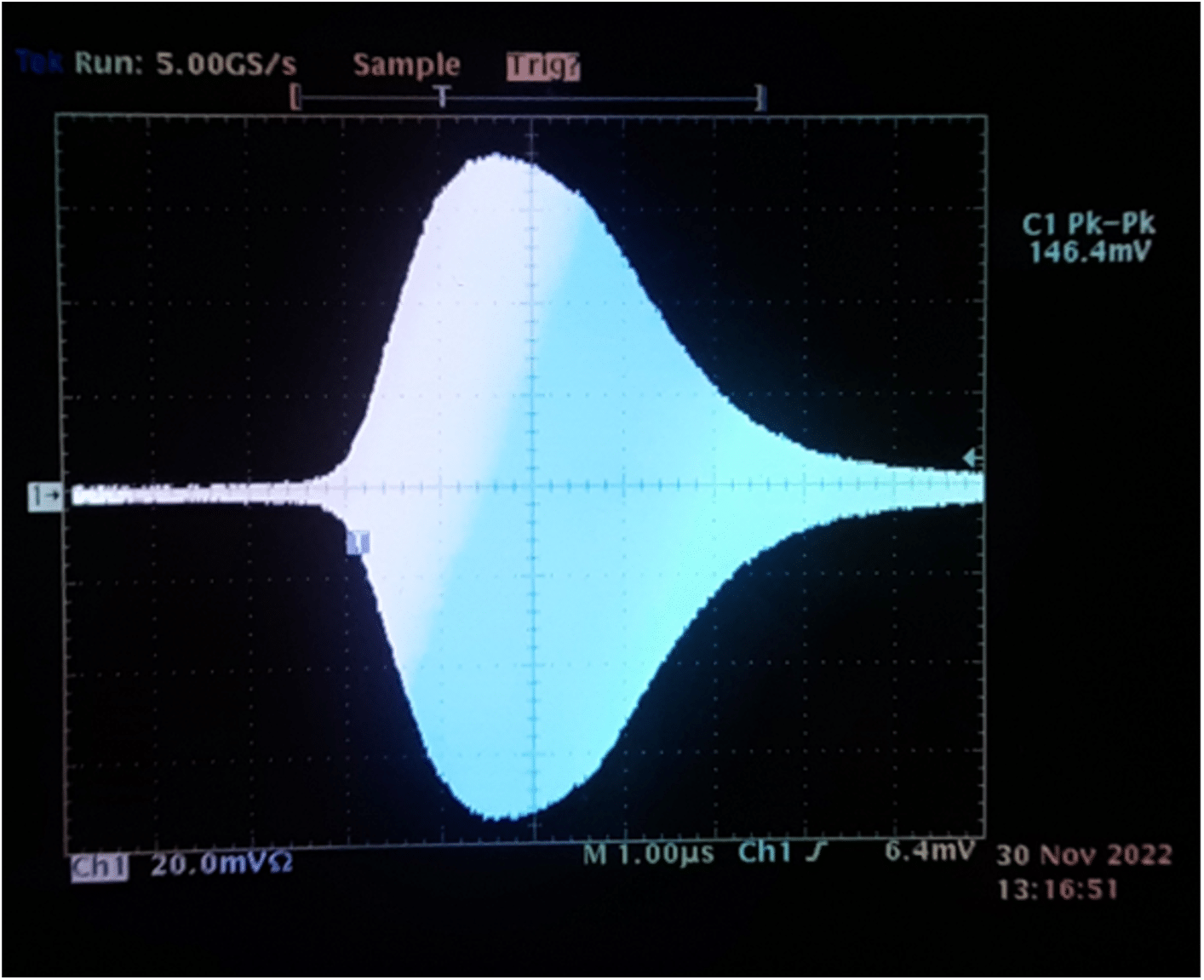
The curve shows a 1MHz to 100MHz 20dBm rated limiter, with a 700MHz input pulse of 30dBm, limited to about 27.3 dBm (~14.6Vpk-pk) at the output, or about 2.7dB compression.

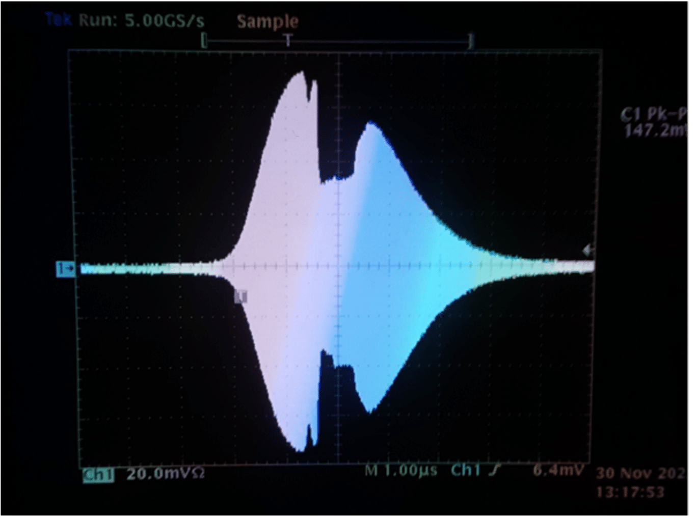
If the 700MHz power is increased to 33dBm, the flat leakage region just begins to form, as shown by the voltage reduction in the middle of the pulse.

The initial response of about 14.6Vpk-pk is followed by a region of about 18.5dBm flat leakage.

Increasing the 700MHz pulse power to 48dBm, the output power pulse magnitude stays nearly constant, however the 18.5 dBm flat leakage duration increases.

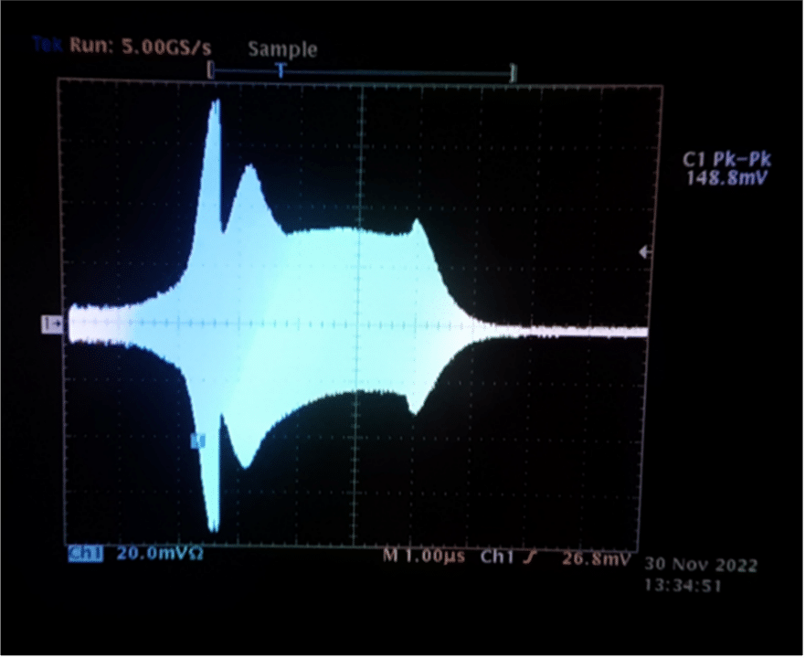
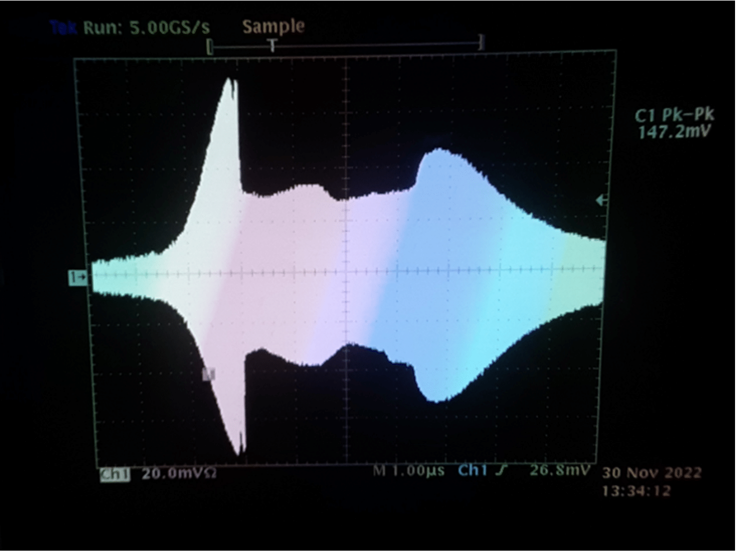
Increasing the 700MHz pulse power further to 50 dBm, the initial spike and flat leakage magnitudes are similar to lower input pulses, but the pulse duration is shorter.

Pulsing the limiter with 50dBm at 2.2GHz, we see an out-put of 21.1dBm. The spike leakage and transition phenomena do not occur at this test condition.

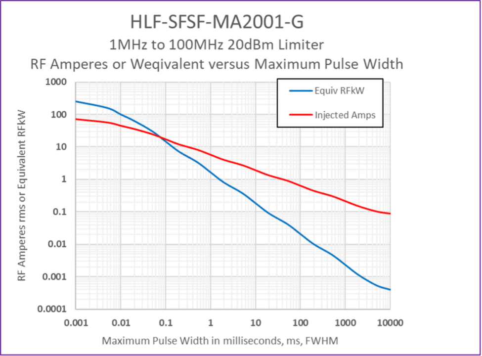
Limiters have a maximum pulse width versus input power level that is primarily a function of power dissipation and resulting temperature rise.

This usually assumes a 25ºC initial temperature. This HF limiter has a maximum power equivalent level over 100kW for pulses less than 10 microseconds.

Figure 12 presents the single pulse power versus maximum pulse width for this device for pulse power above the blue curve, duty cycle effects, or off time, must be used to reduce the average power.

This represents the pulse limitation where off time needs to be used to prevent excessive temperature rise of the limiter. The concept of pulse current is introduced here.

To best capture the quality and effectiveness is to rate the limiter to input current. While the RF power might usually be measured at 50 Ohms, the limiter is not close to 50 Ohms when in the limiting mode.

In addition, RF amplifiers or other sources can usually have much lower impedance than 50 Ohms. Therefore, the current can vary, depending upon the source or generator, and the limiter.

To provide predictable performance, the capacity of the limiter is best related to the input pulse current levels. This figure can also be used to convert RF Watts to Current.

The cumulative effects of a series of several pulse currents needs to be considered and modeled.

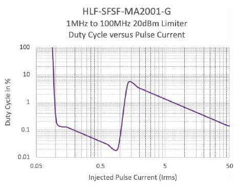
The limiter duty cycle versus injected pulse current is shown in Figure 13.

This graph is another way to view the need to modulate or allow quiescent time for the limiter. Pulse currents must be limited by the duty cycle (the pulse duration divided by the usually longer off time).

The cumulative effects of pulse trains of varying currents and pulse widths needs to be considered and modeled.

SUMMARY

The information presented along with measured lab results provide an introductory explanation of the performance of Nextek’s high-performance HLF series limiters designed for high energy environments.

A systems engineer needs to consider many variables to fully deter-mine the threat level and protection level requirements to ensure the limiter is providing the protection desired.

Direct current injection testing is a good indicator of how a device will perform. Testing across duty cycle, pulse widths, frequency and power levels can be expensive and time consuming.

The results presented in this paper provide a glimpse into what one would expect to see as they do their own testing.